Introduction

Cancer remains a devastating health problem despite modern advances in medicine. Best efforts to fight cancer come with early detection, but testing and screening can be costly, slow, and inconvenient. In order to simplify the process so that more people can be tested more often, machine learning can be used in an attempt to quickly and easily diagnose cancer.

A 2012 study by high schooler Brittany Wenger demonstrated how a multilayer perceptron (MLP) can quite successfully diagnose cancer from fine-needle aspiration¹. Fine-needle aspiration involves no surgery and is one of the simplest means of sampling cells for cancer. On the patient’s end, fine-needle aspiration involves nothing more than a gentle prodding with a fine needle. The needle collects a small sample of cells from a questionable growth, and these cells are dyed and imaged, as shown in the below image².

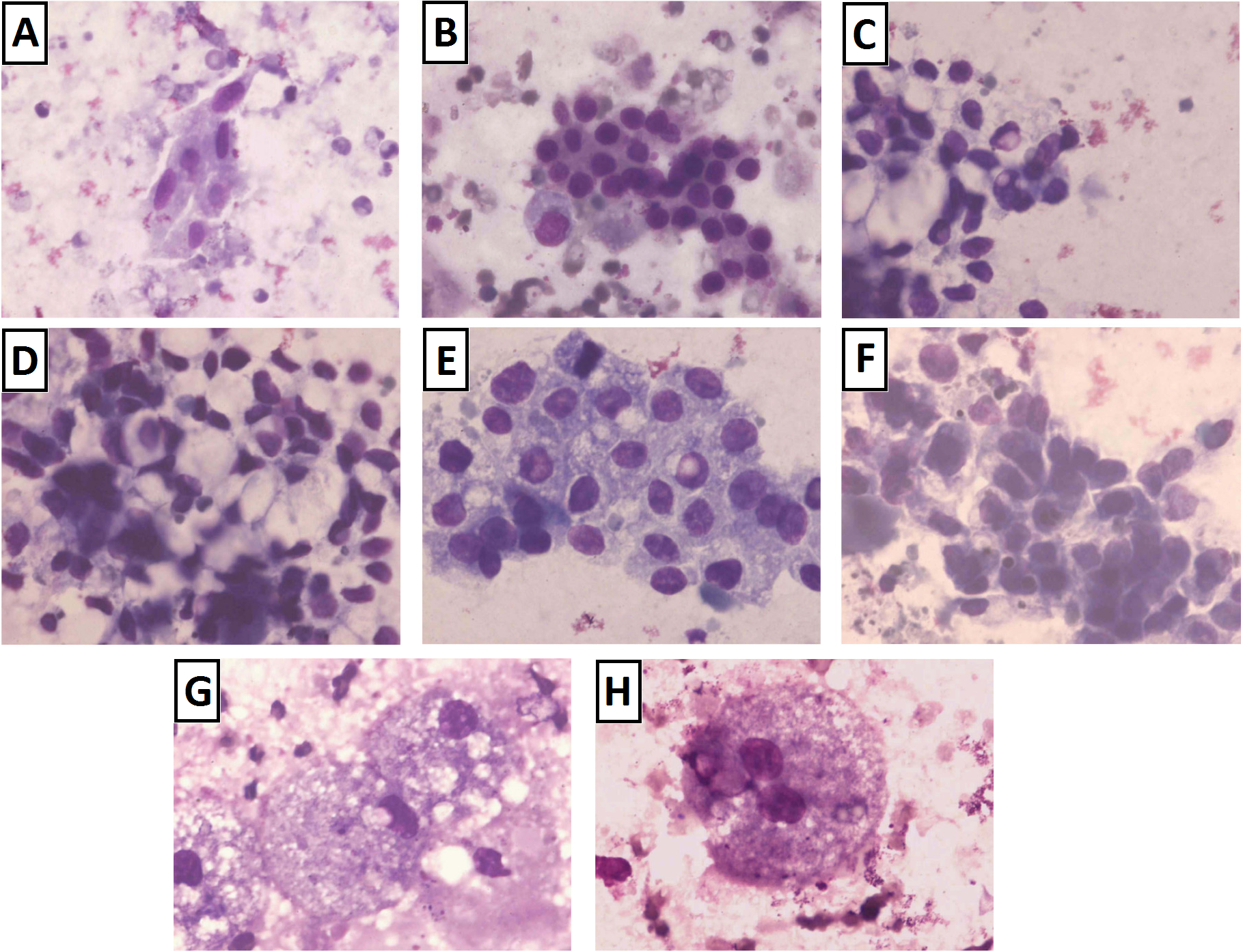
Unfortunately, the simplicity of this procedure makes it is also among the least conclusive procedures for diagnosis. Patterns in images may be difficult to comprehend, with the above image showing only a handful of possibilities. Training a neural network to identify sample characteristics imperceptible to humans could greatly increase the effectiveness of this technique. This would create a simple, effective means of detecting breast cancer, helping deliver the early diagnosis required to save lives.

Brittany’s results are impressive:

	Positive	Negative	Actual
Positive	222	15	93.67%
Inconclusive	14	11	3.67%
Negative	2	417	99.52%
	99.11%	96.53%

There were two shortcomings with Britney’s method. The first of which being 3.67% of samples are unclassified. While this lowers the number of misclassified data, it lowers the usefulness of the model. In the model to be discussed, all data will be classified.

Secondly, this reliability is the result of training on almost the entire data set–all but one sample was used when training. This risks over-fitting of the given data, and her results may not well scale to real-world application. The model derived in this experiment will use a smaller subset of its data to demonstrate better generalization.

In addition to these improvements, a primary goal of this implementation is to maintain a low false negative diagnosis rate. Higher overall accuracy will be sacrificed to prevent wrongfully telling a patient he or she is healthy.

Data Preprocessing

Interpreting Data

The dataset analyzed came from 699 fine-needle aspiration samples. Each sample had up to nine dimensions, covering the following attributes:

1. Clump Thickness

2. Uniformity of Cell Size

3. Uniformity of Cell Shape

4. Marginal Adhesion

5. Single Epithelial Cell Size

6. Bare Nuclei

7. Bland Chromatin

8. Normal Nucleoli

9. Mitoses

Each characteristic was pre-classified on a scale of 1-10, with 10 exhibiting the highest degree of its respective characteristic. This abstraction limited the resolution of available data, but it conveniently normalized all dimensions, preventing any particular dimension from diluting the separability of data.

Dealing with Anomalies

Of the 699 samples, 16 were incomplete, coming from samples in which the number of bare nuclei could not be determined. It became necessary to characterize the data, determining how the incomplete data may affect the overall distribution. First, the mean and variance of both groups was calculated:

Attribute	Complete	Incomplete	Complete	Incomplete
	Mean	Mean	Variance	Variance
1	4.44	3.38	7.96	5.98
2	3.15	2.44	9.40	5.60
3	3.22	2.88	8.93	4.78
4	2.83	1.81	8.21	5.23
3.23	5	2.44	4.94	2.80
6	3.54	N/A	13.28	N/A
7	3.45	3.13	6.00	3.72
8	2.87	2.75	9.32	10.20
9	1.60	1.00	3.00	0.00

Data with higher variance are more spread and better-separable. In other words, higher variance is desireable when aiming to classify data. At a glance, the first noticeable deviation between data sets is that complete samples tend to have higher variance. The parameter with the most variance, “Bare Nuclei,” or number 6, is the attribute incomplete data are missing. It was determined that the incomplete data were far less useful than complete data. In the end, they were discarded.

Analyze Characteristics

Data were further analyzed in order to better conceptualize how cancerous and noncancerous samples may differ. Initially, means and variances of healthy and cancerous samples were calculated:

Attribute	Healthy	Cancerous	Healthy	Cancerous
	Mean	Mean	Variance	Variance
1	2.96	7.19	2.80	5.94
2	1.31	6.58	0.73	7.42
3	1.41	6.56	0.92	6.60
4	1.35	5.59	0.84	10.22
5	2.11	5.33	0.76	5.97
6	1.35	7.63	1.38	9.71
7	2.08	5.97	1.13	5.21
8	1.26	5.86	0.91	11.21
9	1.07	2.60	0.26	6.58

Numerically, trends between cancerous and noncancerous samples are clearly discernable: cancerous samples showed more pronounced characteristics in all regards, with an average of more than double that of noncancerous in every attribute. Because of the high variance in cancerous samples, however, it is very likely that cancerous samples may exist with low values for most parameters. As a result, we determined that nonlinear learning algorithms must be used.

System Hierarchy

Network Determination

A few key characteristics governed development of a large-scale learning algorithm: dimensional significance, natural clustering, and inherent nonlinearity.

Dimensional Significance

The above table illustrates that each characteristic of a sample has a unique differentiation between cancerous and healthy cells. The normalization of the data inherent in its presentation means that more useful differentiators are weighted just as heavily as parameters that may not well divide healthy cells from cancerous cells. Instead of applying a linear weighting to values that seemed significant, experimentation was performed with an MLP learner, as Brittany had used. As an MLP converges to a solution, it adjusts its input weights iteratively in a way that helps the solution form. The success of this method can be seen in the MLP confusion matrix.

Natural Clustering

The above table illustrates a tendency of healthy data to remain clustered in a low-valued region and cancerous data to exist in higher-valued space. The k-Nearest Neighbor (KNN) algorithm was experimented with because of its success in finding clusters. Performance was surprisingly effective, shown in the KNN confusion matrix.

Nonlinearity

Cancerous data were seen with high variance in every parameter. Because of this, data was not entirely linearly separable, and clustering is guaranteed to produce some level of error. By applying various nonlinear transformations to the dataset, it was found that data could be better separable. An MLP displayed good performance overall, with an especially low number of false negatives, shown in the SVM with MLP Kernel confusion matrix. A radial-basis function (RBF) kernel was experimented with, taking advantage of the data’s clustering. Its success is shown in the SVM with RBF confusion matrix. Polynomial transformation was well-rounded in its classification, as shown in the SVM with Polynomial confusion matrix.

System Model

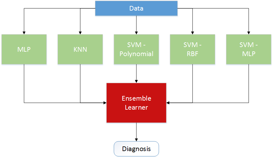
Each of the previous methods were considered, and experiments were performed with all. In the end, the most successful combination incorporated all learners as an ensemble. More precise models tended to be more volatile, and less precise models helped stabilize the system over this variation. The system, shown in the [above image], works nearly as well as its strongest component. Because the strongest component can vary from sample to sample, this method was more consistently reliable than any other. The results of the entire learner are illustrated in the ensemble learner’s confusion matrix

Parameter Calculation

Multiple tests were run in order to figure out the ideal parameters for the supplied data set. The idea behind each of these tests was to train a network on the data set with varying parameters, and determine the configuration with the lowest error. As was discussed earlier, the proposed detection system should focus reducing the number of false negatives, as these have a greater danger to a patient. Therefore, the error during parameter calculation was determined by finding the lowest percentage of false negatives out of the total number of test data.

The parameter variation was done via a brute force method, where every permutation of the different paramters were tried. Training, validation, and testing data were randomly selected for each network in an effort to allow for trustworthy results. In addition to randomized data, multiple iterations were ran for each parameter permutation and the results were normalized each time. From this randomized cross-validation, the performance of each of the network parameters could be used in the final system with confidence.

System Implementation

The implementation of the final system is comprised of three parts: data segmentation, sub-learner training, and ensemble training.

Data Segmentation

Learning and testing are the two general steps which a neural network goes through when given a set of data. The learning step is further split into both training and validation steps. The training step is where the network designs its response to the data, and the validation is then used to check the network’s configuration. This learn-validate step is repeated until a network dependent stop condition is reached. After the stop condition is reached, the testing step uses data which has thus far been unseen by the network, and checks the final response of the network. The important condition is that the data used for testing remain unseen by the network until learning has finished. If this is not met, and the testing data is used in training the system, then the results gathered during the testing phase cannot be trusted as it had a direct effect on the outcome. This would be similar to studying for a test by reading the questions on the test.

Another issue which may arise can be choosing data which doesn’t truly represent the data set as a whole. This will result in training or testing on fringe cases, and will not generalize well. This can be remedied by selecting random data, reducing the probability that outlier data will be selected.

To ensure the data used for testing is not used during training, and no outlier data is selected, the first thing which happens is that the data is randomly split into a training and a testing set. The same training set is used for training each of the sub-learners. Similarly, the testing set is used for determing the performance of the system by feeding the inputs of each of the sub-learners.

Sub-Learners

There are five sub-learners which are used in the final system: a multilayer perceptron, a K-nearest neighbor network, and three support vector machines with different kernel functions. Each of the parameters chosen for the sub-learners was chosen by selecting the best performing configuration as was discussed in the parameter calculation section.

The MLP network was created using the newff command in MATLAB which produces a feed-forward backpropagation network. The chosen setup was three hidden layers each with ten neurons. It was also chosen to use the Levenberg-Marquardt algorithm for training with a μ of 0.046. The output from this learner can be seen in the confusion matrix above.

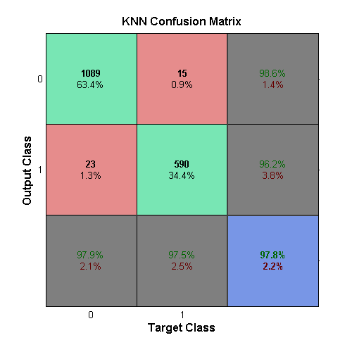
The KNN network was created using the ClassificationKNN.fit command. By default this uses 1 as the number of neighbors needed when classifying. Following the parameter testing, the best performance was found when 5 was used for this parameter. The results for the KNN sub-learner can be seen in the confusion matrix above.

All of the SVMs use the svmtrain function, which creates and trains an SVM network. The first SVM created uses an MLP kernel function. This kernel takes in two parameters, p1 and $$p_2$$, which are used in $$tanh(p_1UV'+p_2)$$. The parameter calculation yielded p1 = 2.1544 and p2 = −3.5938 for best performance, when the box-constraint, C, value was set to 0.001. The figure for this sub-learner can be seen in the confusion matrix above.

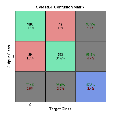
The second SVM uses the radial basis function as its kernel, and takes in a scaling factor, σ, as its parameter. Following the parameter calculation, a value of σ = 7.196857 was chosen along with a box-constraint of 10. The output for this can be seen in the confusion matrix above.

The final SVM uses a polynomial kernel function, which can have a variable order. A 2n**d-order function was deemed best when combined with a box-constraint of 0.01. This output can be seen in the confusion matrix above.

Ensemble

Ensemble learning is performed by using multiple weak learners, boosting them, and turning them strong learners. This type of learning method is used as the final step of the system. The five sub-learners feed their outputs into the ensemble learner, and then discriminant analysis is used train the ensemble.

The purpose of using another learning method to classify based on the outputs of the sub-learners is to have a slightly more robust method of choosing how the different learners actually line up with each other. An example would be if two tend to agree on malignant classifications, however not on benign classifications, it would be smart to use this as a strong indicator of malignant records. The idea is that the final error would be less than (or equal to) each of the sub-learners.

The ensemble learner is created by using the fitensemble method included in MATLAB. This function takes in the number of weak learners used, which was chosen to be 500 as this had a good tradeoff between runtime and performance. The ensemble was trained using the outputs of the sub-learners from the training data set. The performance of the ensemble, and final outputs of the system, was created by using the testing data set piped through the sub-learners and finally to the ensemble. The final output of the system can be seen in the above confusion matrix.

Results and Conclusions

Results are presented as a collection of trials. In order to demonstrate the robustness of this method, random cross-validation was performed. Each learner was trained using 90% of available data, and the remaining 10% were used to evaluate the effectiveness of the learned solution. These random partitions were selected 25 times, allowing the system to be given a wide variety of setups from which to learn. Each iteration’s results is summed, meaning values less than 25 had trials in which no appearances were made. In other words, most of the 25 trials showed no false negatives with the ensemble learner.

In terms of overall classification, the ensemble result performs nearly identically to its strongest component. While in any small set of trials, an individual learner may outperform the ensemble, the ensemble consistently performs well regardless of initial conditions. Individual learners showed more variation whereas the ensemble is more likely to respond well to an entirely new set of data.

In comparison to Brittany’s results, the ensemble performed well:

Category	Brittany’s Results	Ensemble Results
Sensitivity	99.11%	98.0%
Specificity	96.53%	97.6%
Positive Predictive Value	93.67%	95.6%
Inconclusive Rate	3.67%	0%
Negative Predictive Value	99.52%	98.9%
Overall Accuracy	97.4%	97.7%

Inconclusive data are data most likely to be misclassified. Brittany’s omission of these data should have boosted every category. Additionally, her solution learned from 680 of 681 data, boosting its accuracy at the cost of generalization. Despite the sacrifice of performance in this data set, the ensemble performed comparably.

---

1. Wenger, Brittany. Global Neural Network Cloud Service for Breast Cancer. Science Fair 2012 Summary. Google, 27 Nov. 2013. Web. 9 Dec. 2013. ↩︎

2. Kumar et al. Fine Needle Aspiration Cytology. Photograph. 2007. BiomedCentral. http://www.biomedcentral.com/1471-2407/7/180/figure/F2. Web. 12/9/2013. ↩︎